Geometry Optimization
Overview
Geometry Optimization calculations adjust the atomic positions of a molecule to find a stable structure with minimal electronic energy. This is essential for determining equilibrium geometries, transition states, and reaction pathways.
Check the Input and Visualizer section for the allowed input types and how to upload the files.
Modules Available
Three modules are currently available:
DFT - Density Functional Theory (highest accuracy)
GFN2-XTB - Tight-binding semi-empirical method (fast and reasonably accurate)
Hybrid ML model - Fastest and DFT-accurate using machine learning
Hybrid ML Module Input Fields
Upon selecting the Hybrid ML module, following inputs have to be provided:
Total charge of the molecule (e.g., 0)
Spin mulitplicity = 2S+1 (e.g., 1 for singlet)
GFN2-XTB Module Input Fields
If the GFN2-XTB module is selected, the following inputs must be provided:
Total charge of the molecule (e.g., 0)
Spin multiplicity = 2S+1 (e.g., 1 for singlet)
Toggle to include solvent effects
Select a solvent (e.g., water, ethanol)
DFT Module Input Fields
Upon selecting the DFT module, the following inputs must be provided:
Total charge of the molecule (e.g., 0)
Spin multiplicity = 2S+1 (e.g., 1 for singlet)
Toggle to enable constrained optimization (e.g., fix certain bond lengths)
More About Constrained Optimization
See the Constrained Optimization Details section for details on how to freeze or set specific geometric parameters.
Select the basis set family (e.g., Pople, Dunning)
Select the basis set (e.g., 6-31G, 6-31+Gss)
Choose an exchange-correlation functional (e.g., M06)
Toggle to include solvent effects
Select a solvent (e.g., water, ethanol)
Choose the solvation model (e.g., PCM, SMD)
Toggle to enable dispersion correction (e.g., D3BJ)
Choose a dispersion correction model
Constrained Optimization Details
If you want to freeze any bond, angle, or dihedral during optimization, use the following syntax (atom indices are used):
Note : Atom index can not be zero (0)
Freeze a parameter:
- If you wish to fix a bond of your given input then,
freeze
distance 1 2
- If you wish to fix a angle of your given input then,
freeze
angle 1 2 3
- If you wish to fix a dihedral angle of your given input then,
freeze
dihedral 1 2 3 4
- If you want to set a specific value during optimization (distance in angstroms, angles in degrees):
Set a parameter:
- If you wish to fix a bond at specific value in angstroms,
set
distance 1 2 1.0
- If you wish to fix a angle at specific value (value in degree),
set
angle 1 2 3 60.0
- If you wish to fix a dihedral at specific value (value in degree),
set
dihedral 1 2 3 4 120.0
Note
We have LDA, PBE, PBE0, M06, B3LYP, CAM-B3LYP, and WB97X functionals available right now for the GPU calculations.
Finally, click the Run Optimization button to start the simulation.
Output Details
The following options are available to explore and save the results of your geometry optimization:
To see the optimization trajectory, click the “Trajectory View” button at the top left of the visualiser and press “Start”.
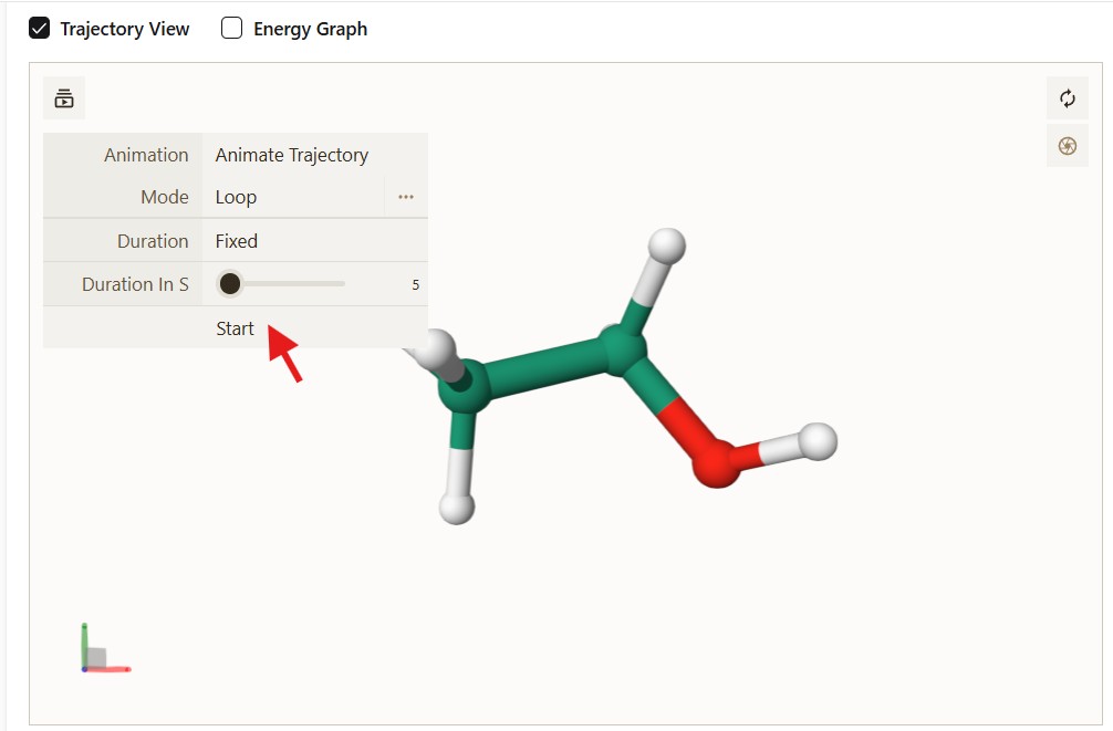
Figure: The Trajectory View interface showing the animation controls.
Click the “Energy Graph” checkbox to display the variation of energy with optimization steps.
In the bottom right corner, you can save the “Trajectory” and “Optimized Structure”. These are in XYZ file format.